Exploring Contextual Effects with merTools

Contextual effects

In a multilevel model, a predictor measured at the individual level can also be aggregated to the group level, and the two can carry different meanings. The classic example is socio-economic status (SES): a student’s own SES captures a within-school relationship, while the average SES of a student’s school captures a contextual (or compositional) effect – the additional influence of attending a more or less advantaged school, over and above a student’s own background.

This vignette reproduces the kind of analysis described in the modelbased package’s article “Studying some effects in context” using the tools in merTools. The data and model follow the contextual-effects example that has long been used to teach multilevel modeling (Raudenbush and Bryk, 2002; Gelman and Hill, 2007).

The data

merTools ships with hsb, a subset of the 1982 High School and Beyond survey: 7,185 students nested in 160 schools. It contains both a student-level SES measure (ses) and the school-mean SES (meanses) – exactly the pair we need to separate within-school and contextual effects.

data(hsb)
str(hsb[, c("schid", "mathach", "ses", "meanses")])

#> 'data.frame':    7185 obs. of  4 variables:
#>  $ schid  : chr  "1224" "1224" "1224" "1224" ...
#>  $ mathach: num  5.88 19.71 20.35 8.78 17.9 ...
#>  $ ses    : num  -1.528 -0.588 -0.528 -0.668 -0.158 ...
#>  $ meanses: num  -0.428 -0.428 -0.428 -0.428 -0.428 -0.428 -0.428 -0.428 -0.428 -0.428 ...

A contextual-effects model

We model math achievement as a function of a student’s own SES and the average SES of their school, allowing each school its own intercept:

cm <- lmer(mathach ~ ses + meanses + (1 | schid), data = hsb)
arm::display(cm)

#> lmer(formula = mathach ~ ses + meanses + (1 | schid), data = hsb)
#>             coef.est coef.se
#> (Intercept) 12.66     0.15  
#> ses          2.19     0.11  
#> meanses      3.68     0.38  
#> 
#> Error terms:
#>  Groups   Name        Std.Dev.
#>  schid    (Intercept) 1.64    
#>  Residual             6.08    
#> ---
#> number of obs: 7185, groups: schid, 160
#> AIC = 46578.6, DIC = 46559
#> deviance = 46563.8

The coefficient on ses is the within-school slope; the coefficient on meanses is the contextual effect. merTools::FEsim() summarizes the uncertainty in both, and plotFEsim() highlights the terms whose interval excludes zero:

fe <- FEsim(cm, n.sims = 500)
plotFEsim(fe) +
  labs(title = "Within-school (ses) vs. contextual (meanses) effects")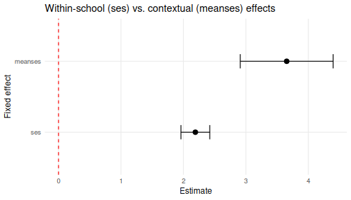

Predictions that separate the two effects

Because meanses enters the model directly, we can ask how the predicted math score changes as we move a student across schools of differing average SES while holding their own SES fixed. wiggle() builds the counterfactual data and predictInterval() attaches prediction intervals:

# A median student in an average school
base_case <- draw(cm, type = "average")
scenarios <- wiggle(base_case, varlist = "meanses",
                    valueslist = list(seq(-0.7, 0.8, by = 0.15)))
pi <- predictInterval(cm, newdata = scenarios, level = 0.9, n.sims = 500,
                      seed = 11213)
scenarios <- cbind(scenarios, pi)

ggplot(scenarios, aes(x = meanses, y = fit, ymin = lwr, ymax = upr)) +
  geom_ribbon(alpha = 0.2) +
  geom_line() +
  labs(x = "School-average SES (context)", y = "Predicted math achievement",
       title = "Contextual effect of school SES (own SES held at its mean)") +
  theme_minimal(base_size = 12)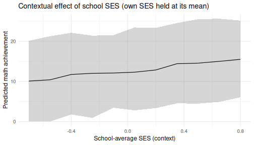

How much do schools matter across the rank distribution?

Finally, REimpact() summarizes how much being in a higher- versus lower-performing school shifts the predicted outcome, binning schools by their expected rank. plotREimpact() (new in this release) plots the result, and can overlay several cases for comparison:

imp <- REimpact(cm, newdata = hsb[1, ], groupFctr = "schid",
                breaks = 4, n.sims = 500)
plotREimpact(imp) +
  labs(title = "Impact of school placement on predicted achievement")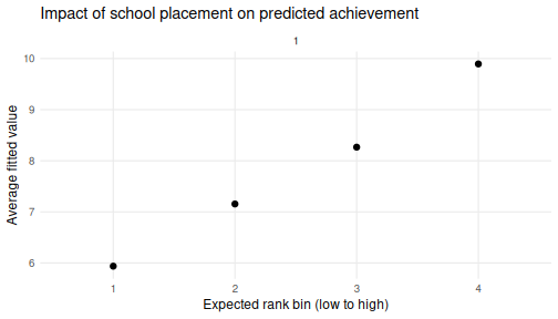

References

Bates, D., Maechler, M., Bolker, B., and Walker, S. (2015). Fitting Linear Mixed-Effects Models Using lme4. Journal of Statistical Software, 67(1), 1-48.

Gelman, A. and Hill, J. (2007). Data Analysis Using Regression and Multilevel/Hierarchical Models. Cambridge University Press.

Lüdecke, D., et al. modelbased: Studying some effects in context. easystats. https://easystats.github.io/modelbased/articles/practical_context_effect.html

Raudenbush, S. W. and Bryk, A. S. (2002). Hierarchical Linear Models: Applications and Data Analysis Methods (2nd ed.). SAGE.