Validating predictInterval() against brms
Jared Knowles
Written 2026-05-29 (last updated 2026-05-29)
Source:vignettes/brms_validation.Rmd
brms_validation.RmdWhy compare to brms?
merTools::predictInterval() was written to put
prediction intervals on mixed-effect models that are too large or too
slow to bootstrap. It does this by simulating from the estimated
distribution of the fixed and random effects – fast, but an
approximation. Since then, brms has become a standard for
fully Bayesian multilevel modeling, and its posterior
predictive distribution is about as close to a gold standard as we have.
This vignette asks a simple question: how close are
predictInterval()’s intervals to the ones brms
produces?
We look at three things: a Gaussian random-slopes model, what happens
for an entirely unobserved group, and a binomial GLMM. This vignette is
precompiled – reproducing it requires the brms
package and a working Stan toolchain.
A random-slopes model
We use the bundled hsb data (7,185 students in 160
schools) and model math achievement from student SES, school-mean SES,
and a school-varying SES slope. We hold out 20% of students for testing,
plus six whole schools to stand in for “new groups” later.
data(hsb)
hsb$schid <- factor(hsb$schid)
new_schools <- sample(levels(hsb$schid), 6)
hsb$.set <- "train"
hsb$.set[hsb$schid %in% new_schools] <- "test_new"
seen <- which(hsb$.set == "train")
hsb$.set[sample(seen, round(0.2 * length(seen)))] <- "test_seen"
train     <- droplevels(hsb[hsb$.set == "train", ])
test_seen <- hsb[hsb$.set == "test_seen" & hsb$schid %in% levels(train$schid), ]
test_new  <- hsb[hsb$.set == "test_new", ]

f1 <- mathach ~ ses + meanses + (ses | schid)
m_lme <- lmer(f1, data = train)
brms_fit_seconds <- system.time(
  m_brm <- fit_brm(f1, train, gaussian(), "brms_hsb_meanses"))[["elapsed"]]
We draw a predictive distribution for each held-out student from each
method – predictInterval(returnSims = TRUE) and
brms::posterior_predict() – and compute everything (point
estimates, intervals, coverage) from those draws.
mt_seen <- mt_draws(m_lme, test_seen)
pp_seen <- posterior_predict(m_brm, newdata = test_seen, allow_new_levels = TRUE)
Point estimates are essentially identical
Both methods condition on the same estimated fixed effects and school BLUPs, so the conditional-mean predictions should agree almost exactly – and they do.
lme_mean <- predict(m_lme, newdata = test_seen)
brm_mean <- colMeans(posterior_epred(m_brm, newdata = test_seen, allow_new_levels = TRUE))
c(correlation = cor(lme_mean, brm_mean),
  mean_abs_diff = mean(abs(lme_mean - brm_mean)),
  response_sd = sd(test_seen$mathach))
#> correlation mean_abs_diff response_sd
#> 0.99984045 0.03670134 6.71745425
ggplot(data.frame(merTools = lme_mean, brms = brm_mean), aes(merTools, brms)) +
  geom_abline(slope = 1, intercept = 0, linetype = 2, color = "grey50") +
  geom_point(alpha = 0.3, size = 0.8, color = "#1B9E77") + coord_equal() +
  labs(x = "lme4 predict()", y = "brms posterior_epred()") +
  theme_minimal(base_size = 12)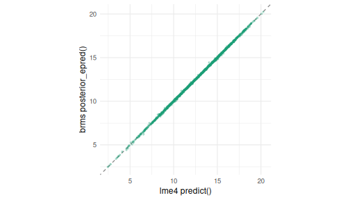
The prediction intervals agree
b_mt <- qband(mt_seen, 0.90); b_brm <- qband(pp_seen, 0.90)
c(width_merTools = median(b_mt$upr - b_mt$lwr),
  width_brms = median(b_brm$upr - b_brm$lwr),
  cor_lower = cor(b_mt$lwr, b_brm$lwr),
  cor_upper = cor(b_mt$upr, b_brm$upr))
#> width_merTools width_brms cor_lower cor_upper
#> 20.1789145 20.2344075 0.9901934 0.9899334
endpts <- rbind(data.frame(bound = "lower", merTools = b_mt$lwr, brms = b_brm$lwr),
                data.frame(bound = "upper", merTools = b_mt$upr, brms = b_brm$upr))
ggplot(endpts, aes(merTools, brms, color = bound)) +
  geom_abline(slope = 1, intercept = 0, linetype = 2, color = "grey50") +
  geom_point(alpha = 0.3, size = 0.8) + coord_equal() +
  labs(title = "90% prediction-interval endpoints", x = "merTools", y = "brms") +
  theme_minimal(base_size = 12)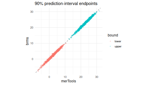
And they are equally well calibrated
The real test is out-of-sample: do nominal intervals cover held-out scores at the nominal rate? Both methods track the diagonal, and each other.
data.frame(nominal = NOMINAL,
           merTools = coverage(mt_seen, test_seen$mathach, NOMINAL),
           brms     = coverage(pp_seen, test_seen$mathach, NOMINAL))
#> nominal merTools brms
#> 1 0.50 0.4569776 0.4598698
#> 2 0.80 0.7895879 0.7932032
#> 3 0.90 0.9168474 0.9168474
#> 4 0.95 0.9660159 0.9703543At a fraction of the cost
t_lme <- system.time(lmer(f1, data = train))[["elapsed"]]
t_mt  <- system.time(mt_draws(m_lme, test_seen))[["elapsed"]]
t_pp  <- system.time(posterior_predict(m_brm, newdata = test_seen,
                                       allow_new_levels = TRUE))[["elapsed"]]
data.frame(  # brms_fit_seconds was captured when the model was fit, above
  step = c("lme4 fit", "predictInterval", "brms fit (compile+sample)", "posterior_predict"),
  seconds = round(c(t_lme, t_mt, brms_fit_seconds, t_pp), 2))
#> step seconds
#> 1 lme4 fit 0.05
#> 2 predictInterval 0.53
#> 3 brms fit (compile+sample) 398.97
#> 4 posterior_predict 1.52For this model, the entire lme4 + predictInterval() path
runs in about a second, while a single brms fit takes several minutes –
a couple of orders of magnitude difference, before the (much larger)
models predictInterval() was really built for.
What about an entirely new group?
For a school that was never seen during fitting there is a genuine modeling choice: do you drop the school’s effect and predict from the fixed effects only, or sample a plausible effect for it from the estimated school-level distribution? Both packages support either, and the comparison is only fair when the choices match:
| treatment of an unseen group | predictInterval() |
brms |
|---|---|---|
| drop the effect (population prediction) |
new.levels = "zero" (default)
|
re_formula = NA |
| sample a new effect | new.levels = "draw" |
allow_new_levels = TRUE (default)
|
Matched up, the two tools agree on both the width and the coverage of the new-school intervals:
nd <- test_new
pp_pop  <- posterior_predict(m_brm, newdata = nd, re_formula = NA)
pp_draw <- posterior_predict(m_brm, newdata = nd, allow_new_levels = TRUE)
mt_zero <- mt_draws(m_lme, nd, new.levels = "zero")
mt_draw <- mt_draws(m_lme, nd, new.levels = "draw")
w <- function(d) median(qband(d, 0.90)$upr - qband(d, 0.90)$lwr)
data.frame(
  unseen_group   = c("drop effect", "sample effect"),
  merTools_width = c(w(mt_zero), w(mt_draw)),
  brms_width     = c(w(pp_pop),  w(pp_draw)),
  merTools_cov90 = c(coverage(mt_zero, nd$mathach, 0.90), coverage(mt_draw, nd$mathach, 0.90)),
  brms_cov90     = c(coverage(pp_pop,  nd$mathach, 0.90), coverage(pp_draw, nd$mathach, 0.90)))
#> unseen_group merTools_width brms_width merTools_cov90 brms_cov90
#> 1 drop effect 19.96801 20.02855 0.8708487 0.8745387
#> 2 sample effect 20.67910 20.76924 0.8892989 0.8856089So the interval width for an unseen group is set by the
choice, not the method. Earlier I compared
predictInterval()’s default against brms’s default, which
is an apples-to-oranges pairing – the apparent “gap” was the two
packages making different default assumptions, not a deficiency in
either.
How much the choice matters depends on how much group variance is
left after the fixed effects. Here meanses already absorbs
most of the between-school variation, so dropping vs. sampling the
school effect barely changes the width. Remove meanses and
the school SD roughly doubles, so the two options diverge:
m0 <- lmer(mathach ~ ses + (ses | schid), data = train)
data.frame(
  model = c("with meanses", "without meanses"),
  school_SD = c(attr(VarCorr(m_lme)$schid, "stddev")[["(Intercept)"]],
                attr(VarCorr(m0)$schid,    "stddev")[["(Intercept)"]]),
  width_zero = c(w(mt_draws(m_lme, nd, new.levels = "zero")),
                 w(mt_draws(m0,    nd, new.levels = "zero"))),
  width_draw = c(w(mt_draws(m_lme, nd, new.levels = "draw")),
                 w(mt_draws(m0,    nd, new.levels = "draw"))))
#> model school_SD width_zero width_draw
#> 1 with meanses 1.598503 19.96801 20.67910
#> 2 without meanses 2.125770 19.94993 21.22576The practical guidance: predictInterval()’s default
(new.levels = "zero") answers “what is the expected outcome
for a typical member of an unseen group,” while
new.levels = "draw" answers “what is the outcome for an
unseen group drawn from the population” – the same quantity brms returns
by default. Pick the one that matches your question.
A generalized linear mixed model
The story carries over to GLMMs. We fit a binomial model for whether
grouse had ticks and compare predicted probabilities –
predictInterval(type = "probability") against
brms::posterior_epred().
data(grouseticks)
grouseticks$TICKS_BIN <- as.integer(grouseticks$TICKS >= 1)
grouseticks$cHEIGHT   <- as.numeric(scale(grouseticks$HEIGHT))
gk <- grouseticks
gk$.set <- ifelse(runif(nrow(gk)) < 0.2, "test", "train")
gk_tr <- droplevels(gk[gk$.set == "train", ])
gk_te <- gk[gk$.set == "test" & gk$BROOD %in% levels(gk_tr$BROOD) &
            gk$LOCATION %in% unique(gk_tr$LOCATION), ]

gf <- TICKS_BIN ~ YEAR + cHEIGHT + (1 | BROOD) + (1 | LOCATION)
g_lme <- glmer(gf, family = binomial, data = gk_tr,
               control = glmerControl(optimizer = "bobyqa"))
g_brm <- fit_brm(gf, gk_tr, bernoulli(), "brms_grouseticks")

mt_pr <- mt_draws(g_lme, gk_te, type = "probability", include.resid.var = FALSE)
if (max(mt_pr) > 1 || min(mt_pr) < 0) mt_pr <- plogis(mt_pr)
brm_pr <- posterior_epred(g_brm, newdata = gk_te, allow_new_levels = TRUE)
mt_p <- apply(mt_pr, 2, median); brm_p <- apply(brm_pr, 2, median)
c(correlation = cor(mt_p, brm_p), mean_abs_diff = mean(abs(mt_p - brm_p)))
#> correlation mean_abs_diff
#> 0.99488587 0.02704796
ggplot(data.frame(merTools = mt_p, brms = brm_p), aes(merTools, brms)) +
  geom_abline(slope = 1, intercept = 0, linetype = 2, color = "grey50") +
  geom_point(alpha = 0.4, color = "#7570B3") + coord_equal(xlim = c(0, 1), ylim = c(0, 1)) +
  labs(title = "Predicted P(tick): merTools vs brms",
       x = "predictInterval(type = 'probability')", y = "posterior_epred()") +
  theme_minimal(base_size = 12)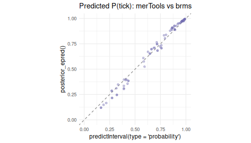
Takeaways
- For observed groups,
predictInterval()reproduces brms’s point estimates and prediction intervals almost exactly, with the same out-of-sample coverage, at a tiny fraction of the computational cost. - For new groups, you choose how to treat the unseen
effect:
new.levels = "zero"(the default) drops it and predicts from the fixed effects, whilenew.levels = "draw"samples it from the estimated covariance – matching brms’sre_formula = NAandallow_new_levels = TRUErespectively. Either way the two packages agree; pick the convention that fits your question. - The same agreement holds for GLMMs on the probability scale.
In short, when bootstrapping or full MCMC is impractical,
predictInterval() is a fast, well-calibrated stand-in for
the cases it was designed to handle.